Differential Expression#
This tutorial covers pseudobulk differential expression: summing each sample’s counts into one profile per cell type, then testing genes for expression differences between conditions. It uses the same Parse Biosciences ~10 million cell PBMC dataset as the other tutorials, comparing IFN-gamma–stimulated cells against PBS controls within each cell type with limma-voom.
Loading and quality control#
Load the data and run QC as in Basic Workflow, keeping the cytokine column that identifies each cell’s treatment. allow_float=True is needed because the raw counts are stored as float32.
from brisc import SingleCell
import polars as pl

sc = SingleCell(
    'Parse_10M_PBMC_cytokines.h5ad', num_threads=-1,
    obs_columns=['sample', 'donor', 'cell_type', 'cytokine'])\
    .qc(allow_float=True)
Pseudobulk aggregation#
pseudobulk() sums the raw counts of all cells that share a sample and cell type. Differential expression then runs on these per-sample profiles rather than on individual cells.
The result is a Pseudobulk dataset, which behaves like a dictionary keyed by cell type. Each cell type has three slots: X, a samples × genes matrix of summed counts; obs, one metadata row per sample; and var, the gene metadata. obs adds a num_cells count and keeps the cell metadata that is constant within each sample, such as donor and cytokine.
We keep only the IFN-gamma and PBS samples. cytokine is an Enum column, so it is cast to a string before is_in to match the plain string values.
pb = sc.pseudobulk('sample', 'cell_type')
pb = pb.filter_obs(pl.col('cytokine').cast(pl.String).is_in(['IFN-gamma', 'PBS']))
print(pb)
Pseudobulk dataset with 18 cell types, each with 22-24 samples (obs) and 40,352 genes (var)
    Cell types: B Intermediate/Memory, B Naive, CD4 Memory, CD4 Naive, CD8 Memory, CD8 Naive, CD14
                 Mono, CD16 Mono, HSPC, ILC, MAIT, NK, NK CD56bright, NKT, Plasmablast, Treg, cDC,
                 pDC
CD14 monocytes, for instance, have a 24 × 40,352 count matrix and one obs row per sample:
print(pb.obs['CD14 Mono'].head())
shape: (5, 4)
┌──────────────────┬───────────┬────────┬───────────┐
│ sample           ┆ num_cells ┆ donor  ┆ cytokine  │
│ ---              ┆ ---       ┆ ---    ┆ ---       │
│ enum             ┆ u32       ┆ enum   ┆ enum      │
╞══════════════════╪═══════════╪════════╪═══════════╡
│ Donor1_IFN-gamma ┆ 2526      ┆ Donor1 ┆ IFN-gamma │
│ Donor1_PBS       ┆ 16690     ┆ Donor1 ┆ PBS       │
│ Donor2_IFN-gamma ┆ 1285      ┆ Donor2 ┆ IFN-gamma │
│ Donor2_PBS       ┆ 9159      ┆ Donor2 ┆ PBS       │
│ Donor3_IFN-gamma ┆ 965       ┆ Donor3 ┆ IFN-gamma │
└──────────────────┴───────────┴────────┴───────────┘
IFN-gamma samples have far fewer cells than PBS samples; the num_cells covariate accounts for this in the model.
Sample-level quality control#
qc() filters out low-quality samples and genes. The default filters are:
<10 cells per sample
Outlier samples — far more zero-count genes than average (more than 3 standard deviations above the mean)
Genes detected in <80% of samples
Passing cytokine as the grouping column requires the gene filter to pass within each condition, not just across all samples pooled together.
pb = pb.qc('cytokine')
[B Intermediate/Memory] Starting with 24 samples and 40,352 genes.
[B Intermediate/Memory] Applying the custom filter...
[B Intermediate/Memory] Filtering to samples with at least 10 B Intermediate/Memory cells...
[B Intermediate/Memory] 24 samples remain after filtering to samples with at least 10 B Intermediate/Memory cells.
[B Intermediate/Memory] Filtering to samples where the number of genes with 0 counts is <3 standard deviations above the mean...
[B Intermediate/Memory] 24 samples remain after filtering to samples where the number of genes with 0 counts is <3 standard deviations above the mean.
[B Intermediate/Memory] Filtering to genes with at least one count in 80.0% of samples in each group...
[B Intermediate/Memory] 14,696 genes remain after filtering to genes with at least one count in 80.0% of samples in each group.

...

[Plasmablast] Starting with 22 samples and 40,352 genes.
[Plasmablast] Applying the custom filter...
[Plasmablast] Filtering to samples with at least 10 Plasmablast cells...
[Plasmablast] 11 samples remain after filtering to samples with at least 10 Plasmablast cells.
[Plasmablast] Skipping this cell type because it has only 1 sample where group_column = 'IFN-gamma' after filtering, which is fewer than min_samples (2)

...
QC runs independently for each cell type, so the gene count it keeps varies, and a rare type can drop out entirely when a condition is left with too few samples — here Plasmablast is skipped because only one IFN-gamma sample has enough cells.
Differential expression#
library_size() computes a TMM-normalized library size per sample, and DE() then fits a limma-voom model for each cell type.
The formula ~ 0 + cytokine + donor + log2(num_cells) + log2(library_size) describes each gene’s expression: cytokine is the effect of interest (the leading 0 + drops the intercept so each condition gets its own coefficient), donor accounts for the paired donors, and log2(num_cells) and log2(library_size) — recommended for every pseudobulk model — correct for the number of cells aggregated and for sequencing depth. The contrasts argument asks for the IFN-gamma minus PBS difference.
pb = pb.library_size()
de = pb.DE(
    '~ 0 + cytokine + donor + log2(num_cells) + log2(library_size)',
    contrasts={'IFN-gamma_vs_PBS': '`cytokineIFN-gamma` - `cytokinePBS`'},
    group='cytokine',
    categorical_columns=['donor', 'cytokine'])
donor and cytokine load as Enum columns, which brisc treats as ordered factors. Listing them in categorical_columns switches them to standard treatment coding, which gives the coefficients the readable names (cytokineIFN-gamma, cytokinePBS) referenced in the contrast. group='cytokine' fits the mean–variance trend separately for each condition (voomByGroup), recommended when groups differ in overall expression.
The result is a DE object whose table holds one row per gene per cell type, with the fold change, confidence interval, and corrected p-values:
print(de.table.head())
shape: (5, 11)
┌───────────────────────┬──────────────────┬──────────┬───────────┬──────────┬───────────┬───────────┬──────────┬──────────┬────────────┬──────────┐
│ cell_type             ┆ coefficient      ┆ gene     ┆ logFC     ┆ SE       ┆ LCI       ┆ UCI       ┆ AveExpr  ┆ p        ┆ Bonferroni ┆ FDR      │
│ ---                   ┆ ---              ┆ ---      ┆ ---       ┆ ---      ┆ ---       ┆ ---       ┆ ---      ┆ ---      ┆ ---        ┆ ---      │
│ str                   ┆ str              ┆ str      ┆ f64       ┆ f64      ┆ f64       ┆ f64       ┆ f64      ┆ f64      ┆ f64        ┆ f64      │
╞═══════════════════════╪══════════════════╪══════════╪═══════════╪══════════╪═══════════╪═══════════╪══════════╪══════════╪════════════╪══════════╡
│ B Intermediate/Memory ┆ IFN-gamma_vs_PBS ┆ DPM1     ┆ 0.222663  ┆ 0.641413 ┆ -1.138223 ┆ 1.583548  ┆ 5.572128 ┆ 0.733054 ┆ 1.0        ┆ 0.960307 │
│ B Intermediate/Memory ┆ IFN-gamma_vs_PBS ┆ SCYL3    ┆ 0.058436  ┆ 0.85565  ┆ -1.756998 ┆ 1.87387   ┆ 5.475793 ┆ 0.946406 ┆ 1.0        ┆ 0.993482 │
│ B Intermediate/Memory ┆ IFN-gamma_vs_PBS ┆ C1orf112 ┆ 0.808702  ┆ 0.780593 ┆ -0.847482 ┆ 2.464886  ┆ 5.03358  ┆ 0.31576  ┆ 1.0        ┆ 0.879665 │
│ B Intermediate/Memory ┆ IFN-gamma_vs_PBS ┆ FGR      ┆ -3.817447 ┆ 1.210963 ┆ -6.386748 ┆ -1.248147 ┆ 3.942816 ┆ 0.006227 ┆ 1.0        ┆ 0.694034 │
│ B Intermediate/Memory ┆ IFN-gamma_vs_PBS ┆ FUCA2    ┆ -0.737734 ┆ 1.348779 ┆ -3.599441 ┆ 2.123972  ┆ 3.232465 ┆ 0.592028 ┆ 1.0        ┆ 0.946363 │
└───────────────────────┴──────────────────┴──────────┴───────────┴──────────┴───────────┴───────────┴──────────┴──────────┴────────────┴──────────┘
Note
For a single design term,
coefficient=reports DE for that coefficient directly, instead ofcontrasts.group=Falseuses a single mean–variance trend (plain voom) rather than voomByGroup.robust=Truemakes the empirical Bayes step robust to outlier samples.formulacan be a dict mapping cell types to different formulas when a covariate applies only to some.
Exploring the results#
get_num_hits() counts the significant genes (FDR < 0.05) in each cell type; cell types with no hits are omitted.
print(de.get_num_hits())
shape: (5, 2)
┌───────────────────────┬──────────┐
│ cell_type             ┆ num_hits │
│ ---                   ┆ ---      │
│ str                   ┆ u32      │
╞═══════════════════════╪══════════╡
│ B Intermediate/Memory ┆ 1        │
│ B Naive               ┆ 419      │
│ CD14 Mono             ┆ 921      │
│ CD16 Mono             ┆ 1242     │
│ pDC                   ┆ 8        │
└───────────────────────┴──────────┘
The monocytes and B cells respond most strongly, as expected for IFN-gamma; the other tested cell types show no hits at this threshold.
get_hits() returns the hits themselves; num_top_hits keeps the strongest few per cell type.
print(de.get_hits(num_top_hits=5))
shape: (21, 11)
┌───────────────────────┬──────────────────┬──────────┬───────────┬──────────┬───────────┬───────────┬──────────┬──────────┬────────────┬──────────┐
│ cell_type             ┆ coefficient      ┆ gene     ┆ logFC     ┆ SE       ┆ LCI       ┆ UCI       ┆ AveExpr  ┆ p        ┆ Bonferroni ┆ FDR      │
│ ---                   ┆ ---              ┆ ---      ┆ ---       ┆ ---      ┆ ---       ┆ ---       ┆ ---      ┆ ---      ┆ ---        ┆ ---      │
│ str                   ┆ str              ┆ str      ┆ f64       ┆ f64      ┆ f64       ┆ f64       ┆ f64      ┆ f64      ┆ f64        ┆ f64      │
╞═══════════════════════╪══════════════════╪══════════╪═══════════╪══════════╪═══════════╪═══════════╪══════════╪══════════╪════════════╪══════════╡
│ B Intermediate/Memory ┆ IFN-gamma_vs_PBS ┆ TENM4    ┆ -6.541455 ┆ 0.932481 ┆ -8.5199   ┆ -4.563009 ┆ 5.045181 ┆ 0.000003 ┆ 0.045421   ┆ 0.045421 │
│ B Naive               ┆ IFN-gamma_vs_PBS ┆ LAP3     ┆ 7.407232  ┆ 1.310548 ┆ 4.623667  ┆ 10.190797 ┆ 7.001164 ┆ 0.000039 ┆ 0.59715    ┆ 0.00686  │
│ B Naive               ┆ IFN-gamma_vs_PBS ┆ CASP10   ┆ 5.912959  ┆ 1.276394 ┆ 3.201936  ┆ 8.623982  ┆ 6.22115  ┆ 0.000293 ┆ 1.0        ┆ 0.021485 │
│ B Naive               ┆ IFN-gamma_vs_PBS ┆ CFLAR    ┆ 3.227135  ┆ 0.690015 ┆ 1.761564  ┆ 4.692705  ┆ 8.286078 ┆ 0.000268 ┆ 1.0        ┆ 0.020962 │
│ B Naive               ┆ IFN-gamma_vs_PBS ┆ NFIX     ┆ 4.034178  ┆ 0.959142 ┆ 1.996989  ┆ 6.071367  ┆ 3.726182 ┆ 0.000702 ┆ 1.0        ┆ 0.034705 │
│ B Naive               ┆ IFN-gamma_vs_PBS ┆ REV3L    ┆ -2.426383 ┆ 0.598103 ┆ -3.696736 ┆ -1.15603  ┆ 7.312945 ┆ 0.000956 ┆ 1.0        ┆ 0.040087 │
│ CD14 Mono             ┆ IFN-gamma_vs_PBS ┆ CFH      ┆ 8.41647   ┆ 1.744176 ┆ 4.629897  ┆ 12.203043 ┆ 3.082947 ┆ 0.000378 ┆ 1.0        ┆ 0.028114 │
│ CD14 Mono             ┆ IFN-gamma_vs_PBS ┆ LAP3     ┆ 5.340517  ┆ 0.984571 ┆ 3.203031  ┆ 7.478003  ┆ 9.694517 ┆ 0.000137 ┆ 1.0        ┆ 0.024299 │
│ CD14 Mono             ┆ IFN-gamma_vs_PBS ┆ HS3ST1   ┆ -6.472272 ┆ 1.52021  ┆ -9.772619 ┆ -3.171925 ┆ 2.661385 ┆ 0.001035 ┆ 1.0        ┆ 0.037717 │
│ CD14 Mono             ┆ IFN-gamma_vs_PBS ┆ CASP10   ┆ 3.927577  ┆ 0.694199 ┆ 2.420484  ┆ 5.434671  ┆ 6.461136 ┆ 0.000094 ┆ 1.0        ┆ 0.022213 │
│ CD14 Mono             ┆ IFN-gamma_vs_PBS ┆ CD38     ┆ 9.55195   ┆ 1.940199 ┆ 5.339815  ┆ 13.764086 ┆ 8.810696 ┆ 0.000319 ┆ 1.0        ┆ 0.027588 │
│ CD16 Mono             ┆ IFN-gamma_vs_PBS ┆ C1orf112 ┆ -1.851876 ┆ 0.496937 ┆ -2.910966 ┆ -0.792787 ┆ 4.496459 ┆ 0.002022 ┆ 1.0        ┆ 0.032473 │
│ CD16 Mono             ┆ IFN-gamma_vs_PBS ┆ GCLC     ┆ 2.931873  ┆ 0.673918 ┆ 1.495595  ┆ 4.368152  ┆ 7.405133 ┆ 0.000569 ┆ 1.0        ┆ 0.017878 │
│ CD16 Mono             ┆ IFN-gamma_vs_PBS ┆ LAP3     ┆ 2.727377  ┆ 0.451244 ┆ 1.765669  ┆ 3.689084  ┆ 9.924472 ┆ 0.000022 ┆ 0.313044   ┆ 0.005159 │
│ CD16 Mono             ┆ IFN-gamma_vs_PBS ┆ TMEM176A ┆ 1.858929  ┆ 0.472315 ┆ 0.852313  ┆ 2.865544  ┆ 4.429607 ┆ 0.001319 ┆ 1.0        ┆ 0.026377 │
│ CD16 Mono             ┆ IFN-gamma_vs_PBS ┆ CASP10   ┆ 1.477641  ┆ 0.385716 ┆ 0.655589  ┆ 2.299694  ┆ 6.820638 ┆ 0.001633 ┆ 1.0        ┆ 0.029325 │
│ pDC                   ┆ IFN-gamma_vs_PBS ┆ CALCRL   ┆ 2.570484  ┆ 0.371683 ┆ 1.757332  ┆ 3.383635  ┆ 7.461197 ┆ 0.000019 ┆ 0.189731   ┆ 0.035574 │
│ pDC                   ┆ IFN-gamma_vs_PBS ┆ CD83     ┆ 2.328595  ┆ 0.340925 ┆ 1.582735  ┆ 3.074455  ┆ 7.666968 ┆ 0.000022 ┆ 0.213442   ┆ 0.035574 │
│ pDC                   ┆ IFN-gamma_vs_PBS ┆ IFIT2    ┆ 2.561409  ┆ 0.373712 ┆ 1.743818  ┆ 3.379001  ┆ 6.730806 ┆ 0.000021 ┆ 0.206565   ┆ 0.035574 │
│ pDC                   ┆ IFN-gamma_vs_PBS ┆ GBP5     ┆ 4.729849  ┆ 0.597065 ┆ 3.423617  ┆ 6.036082  ┆ 6.351485 ┆ 0.000005 ┆ 0.050837   ┆ 0.016946 │
│ pDC                   ┆ IFN-gamma_vs_PBS ┆ CXCL10   ┆ 5.11896   ┆ 0.775682 ┆ 3.421958  ┆ 6.815962  ┆ 6.030659 ┆ 0.00003  ┆ 0.294685   ┆ 0.037911 │
└───────────────────────┴──────────────────┴──────────┴───────────┴──────────┴───────────┴───────────┴──────────┴──────────┴────────────┴──────────┘
Classic interferon-response genes recur across cell types — LAP3, GBP5, IFIT2, and CXCL10 are all canonical IFN-gamma targets.
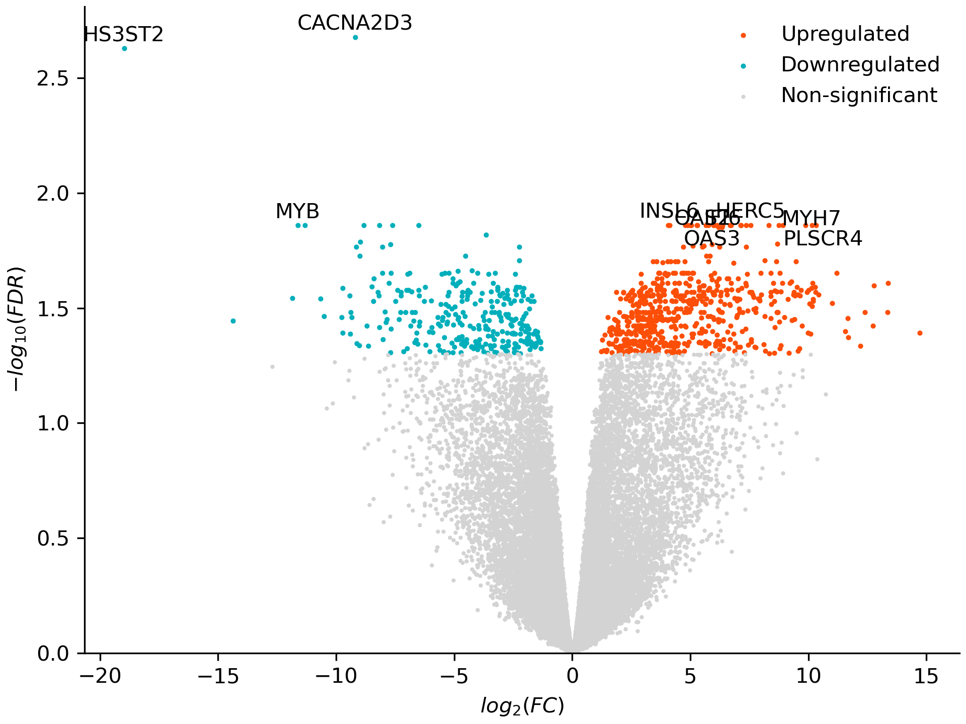
plot_volcano() plots fold change against significance for one cell type. CD14 monocytes mount one of the strongest responses to IFN-gamma:
de.plot_volcano('CD14 Mono', 'volcano.png', significance_column='FDR',
                ylabel='$-log_{10}(FDR)$')
Note
plot_voom()draws the mean–variance trend that voom fits, with one curve per group.significance_column='Bonferroni'or a lowerthresholdinget_hitsandplot_volcanogives a stricter cut.
Pipeline summary#
The full differential expression pipeline:
from brisc import SingleCell
import polars as pl

sc = SingleCell(
    'Parse_10M_PBMC_cytokines.h5ad', num_threads=-1,
    obs_columns=['sample', 'donor', 'cell_type', 'cytokine'])\
    .qc(allow_float=True)

pb = sc.pseudobulk('sample', 'cell_type')\
    .filter_obs(pl.col('cytokine').cast(pl.String).is_in(['IFN-gamma', 'PBS']))\
    .qc('cytokine')\
    .library_size()

de = pb.DE(
    '~ 0 + cytokine + donor + log2(num_cells) + log2(library_size)',
    contrasts={'IFN-gamma_vs_PBS': '`cytokineIFN-gamma` - `cytokinePBS`'},
    group='cytokine',
    categorical_columns=['donor', 'cytokine'])

de.plot_volcano('CD14 Mono', 'volcano.png', significance_column='FDR',
                ylabel='$-log_{10}(FDR)$')
Step |
Method |
What it does |
|---|---|---|
Quality control |
Filter low-quality cells (float32 counts) |
|
Pseudobulk |
Sum raw counts per sample × cell type |
|
Filter conditions |
Keep IFN-gamma and PBS samples only |
|
Sample QC |
Filter low-coverage samples and genes per group |
|
Library size |
TMM-normalized library sizes |
|
Differential expression |
limma-voom with voomByGroup per cell type |
|
Volcano plot |
Fold change vs −log₁₀(FDR) for one cell type |